GPUs Part 2 - Understanding the GPU programming model
Written by Romit Jain
Part 1 in the series gives a basic understanding of the GPU hardware. This blog will describe the programming model that is used to run programs on GPUs.
Hardware to software mapping and programming model of the GPU
2 things to keep in mind before we start:
- The physical concepts of hardware do not necessarily translate one-to-one to logical concepts in software.
- In GPU programming, a kernel is a function that is written to be executed on the GPU. A program can have multiple kernels and they can be “launched” from the CPU.
Threads
Each kernel is executed by a thread in the GPU. And every thread executes the same kernel (assuming there is only a single kernel in the program). This makes it necessary to write kernels such that a single function can operate on all the data points. When a kernel is launched, multiple GPU threads are spawned that execute instructions written inside that kernel. The number of threads that are spawned at once is configurable.
All threads have some small memory associated with it which is called local memory. Apart from that, threads can also access the shared memory, L2 cache, and global memory.
Physically, threads are assigned to cores. Cores execute software threads.
Blocks
Threads are logically organized into blocks. Every block has a pre-defined number of threads assigned to it. Just for logical purposes, threads can be arranged inside a block in either a 1D, 2D, or 3D array layout. Blocks can be thought of as an array of threads. It’s important to understand that this 1D, 2D, or 3D arrangement is purely logical and for the developer’s convenience only. This arrangement is provided so it’s easier to visualize input and output data. For example, if the kernel needs to operate on a 100x100 matrix, then a kernel with a block size of 100 by 100 threads can be launched. That will start a total of $10^4$ (100x100) threads which can be mapped to the matrix. The kernel can be written such that every single thread operates on every single element of the matrix.
In the physical world, every block is assigned an SM (Streaming multiprocessor). Throughout its execution, the block will only be executed on the same SM. Since every block is assigned an SM, it also has access to the SM’s shared memory (refer to Part 1 of the series for more context). All the threads that are part of a single block can access and share this memory.
Grids
Similar to how threads are organized in blocks, blocks are themselves organized into a grid. That allows the GPU to launch multiple blocks at one time. A single GPU has multiple SMs, so multiple blocks can be launched at once so that all of the SMs and cores are utilized. Let’s assume that the program executes 25 blocks and the GPU has 10 SMs. Then the program will execute 10 blocks in the first wave, 10 blocks in the second wave, and 5 blocks in the third wave. The first two waves will have 100% optimization but the last wave will have 50% utilization.
Blocks inside a grid can be organized in the same way that threads are organized inside a block. A grid can have a 1D, 2D, or 3D array layout of the blocks. The arrangement of blocks and threads is just logical. A single program only executes a single grid at a time. The grid has access to the global memory or HBM of the GPU.
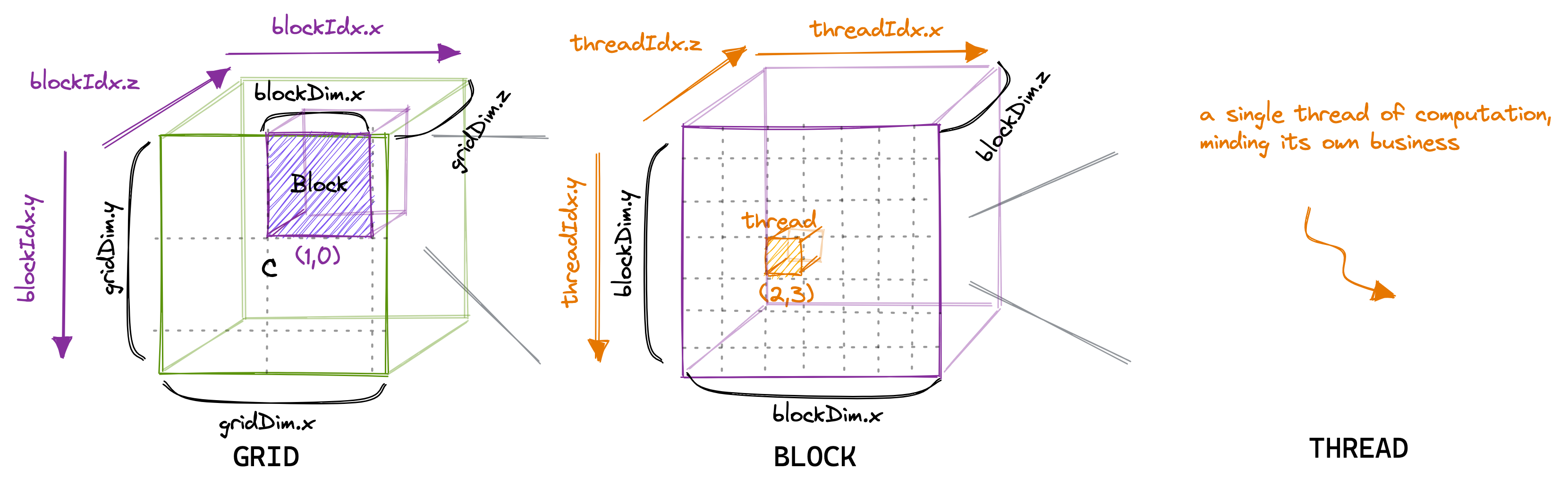
Figure 1: Grids/Blocks/Threads layout Source: Borrowed from this excellent blog.
During execution, a total of blocks per thread (b) * number of blocks (num) physical threads are spawned. Each physical thread is numbered from 0 to (b*num)-1. So, how is the 2D or 3D structure of logical thread blocks mapped to the physical thread? By unrolling.
A 2D array layout can be unrolled to 1D. If it’s row-major ordering, then a 2D matrix after unrolling will look like this:
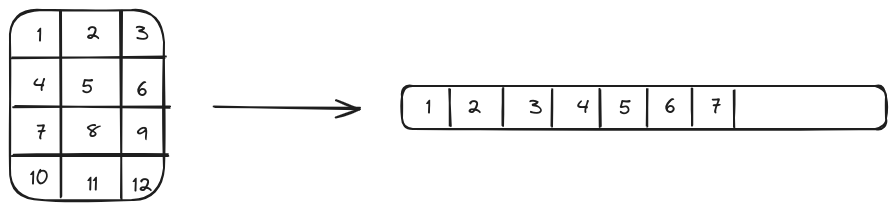
Figure 2: Element A[2][3] in the 2D matrix will be A[5] in the flattened 1D array. This is how the mapping of 2D blocks of thread to the 1D thread array is accomplished.
When blocks and threads are arranged in this 1D, 2D, or 3D layout, CUDA maps them to the x-axis, y-axis, and z-axis in its programming model. This will be useful in the next section.
A simple example in CUDA
CUDA is a programming extension of C/C++ that helps write heterogeneous programs (that run on CPU and GPU). These programs allow to define and launch kernels from the CPU. CUDA is very powerful and offers a lot of ways to optimize the kernels. It’s just a bit … too verbose. Let’s implement a very naive implementation of matrix multiplication to understand how CUDA works. A few CUDA function calls will be used throughout the code. They should be self-explanatory, but in case they are not, just google the syntax. This is a relatively simple kernel, so should be easy to follow along.
Here are the general steps of writing and launching a kernel from CUDA:
- Allocate the memory for the data (both input and output) on the CPU memory (also called as host). Allocate memory for the input (
X), weight matrix (W), and output (O). AssumingBas the batch size,Nas the number of rows or sequence length in transformers,D_inas the number of columns or embedding dimension, and D_out as the hidden dimension.
float *X = (float*)malloc(B*N*D_in*sizeof(float));      // Input data
float *W = (float*)malloc(D_in*D_out*sizeof(float));    // Weights
float *O = (float*)malloc(B*N*D_out*sizeof(float));     // Output data
- Allocate the memory for the data on the GPU (also called as device)
float *d_X, *d_W, *d_O;

cudaMalloc((void**) &d_X, B*N*D_in*sizeof(float));      //cudaMalloc is a CUDA function and allocates memory on the GPU memory
cudaMalloc((void**) &d_W, D_in*D_out*sizeof(float));
cudaMalloc((void**) &d_O, B*N*D_out*sizeof(float));
- Copy the relevant data from the CPU memory to the GPU memory. Let’s assume
XandWare loaded with the relevant data. Next, transfer that data to the GPU. Just for convenience, I have prefixed the variable that will reside on GPU memory withd_. These variables are a copy ofXandWbut allocated in the GPU memory.
cudaMemcpy(d_X, X, B*N*D_in*sizeof(float), cudaMemcpyHostToDevice);     // cudaMemcpy is again a CUDA function
cudaMemcpy(d_W, W, D_in*D_out*sizeof(float), cudaMemcpyHostToDevice);
- Launch the kernel. Assuming that the kernel is called
matMul,griddefines how the blocks are arranged andblocksdefine how threads are arranged in each block. For this example, thegridwill be a 1D array equal to the batch size.blockswill have the same layout as the output dimension of the output matrix (N*D_out). This means that every block will process a single output matrix from the batch and every thread will process a single cell of the output matrix.
// Launch B blocks, each block processing a single batch
dim3 grid(B);
/*
Arrange the threads inside a block in the same dimension as the output
i.e N*D_out, so that logically each thread corresponds to a single element in the
output matrix. Hence, each thread is responsible for computing a single element of the output.
*/
dim3 blocks(D_out, N); //D_out is first instead of N, because the function dim3 takes input in x, y, z notation. x axis is the columnar axis and y axis is the row axis

matMul<<<grid, blocks>>>(
    d_X,
    d_W,
    d_O,
    B,
    N,
    D_in,
    D_out
);
In total B*N*D_out threads are spawned, arranged in B blocks.
- Copy the relevant data (usually only the output) from the GPU memory to the CPU memory. Once the kernel execution is completed, the output is copied from the GPU memory back to the CPU memory so that it can be used for any downstream processing.
cudaMemcpy(O, d_O, B*N*D_out*sizeof(float), cudaMemcpyDeviceToHost);
These 5 steps are followed in almost all GPU programs. Let’s now dive deep into the actual kernel:
__global__ void matMul(
    float* X,
    float* W,
    float* OO,
    int B,
    int N,
    int D_in,
    int D_out
) {
    /*
    This kernel takes a batch of data: (B x N x Din)
    and a weight matrix: (Din X Dout)
    and produces: (B x N x Dout)
    */

    int batch = blockIdx.x;
    int row = threadIdx.y;
    int col = threadIdx.x;

    int out_offset = N*D_out*batch + row*D_out + col;

    if ((batch < B) && (col < D_out) && (row < N)) {
        float sum = 0.0f;
        for (int i = 0; i < D_in; i++) {
            sum += X[N * D_in * batch + row * D_in + i] * W[i * D_out + col];
        }
        OO[out_offset] = sum;
    }
}
Remember that physically there is no 2D or 3D arrangement of threads. That construct is just provided by CUDA to help developers map the problems appropriately. Physically it’s just a single 1D array of threads. Since B*N*D_out threads are spawned, it maps exactly with the 1D layout of the output matrix.
To figure out which data a particular thread should process, the kernel just needs to figure out which thread is it executing. Depending on the batch, row, and column, each thread will load different parts of the input and weight matrix. These are called offsets and there are 4 offsets calculated in the code:
batch: Figure out which matrix in the batch this kernel is processing.blockIdx.xgives the block ID in the x-axis of the grid layout. Since there is a 1D grid, this is the only direction available.row: Figure out within a matrix, which row is the kernel processing. Rows are mapped to the y-axis of the block layout.col: Figure out within a matrix, which column is the kernel processing. Columns are mapped to the x-axis of the block layout.out_offset: Finally, map the thread ID to the exact cell in the output matrix:- Skipping
batchmatrices to arrive at the current matrix. To skip one single matrix, move aheadN*D_outnumber of elements in the flattened 1D array - Skipping
rownumber of rows. In a 1D flattened layout, a row can be skipped by moving aheadD_outelements. - Finally, adding
colto the summation of the above two to arrive at the element.
- Skipping
Hopefully, this figure will make it clearer about the offset calculation.
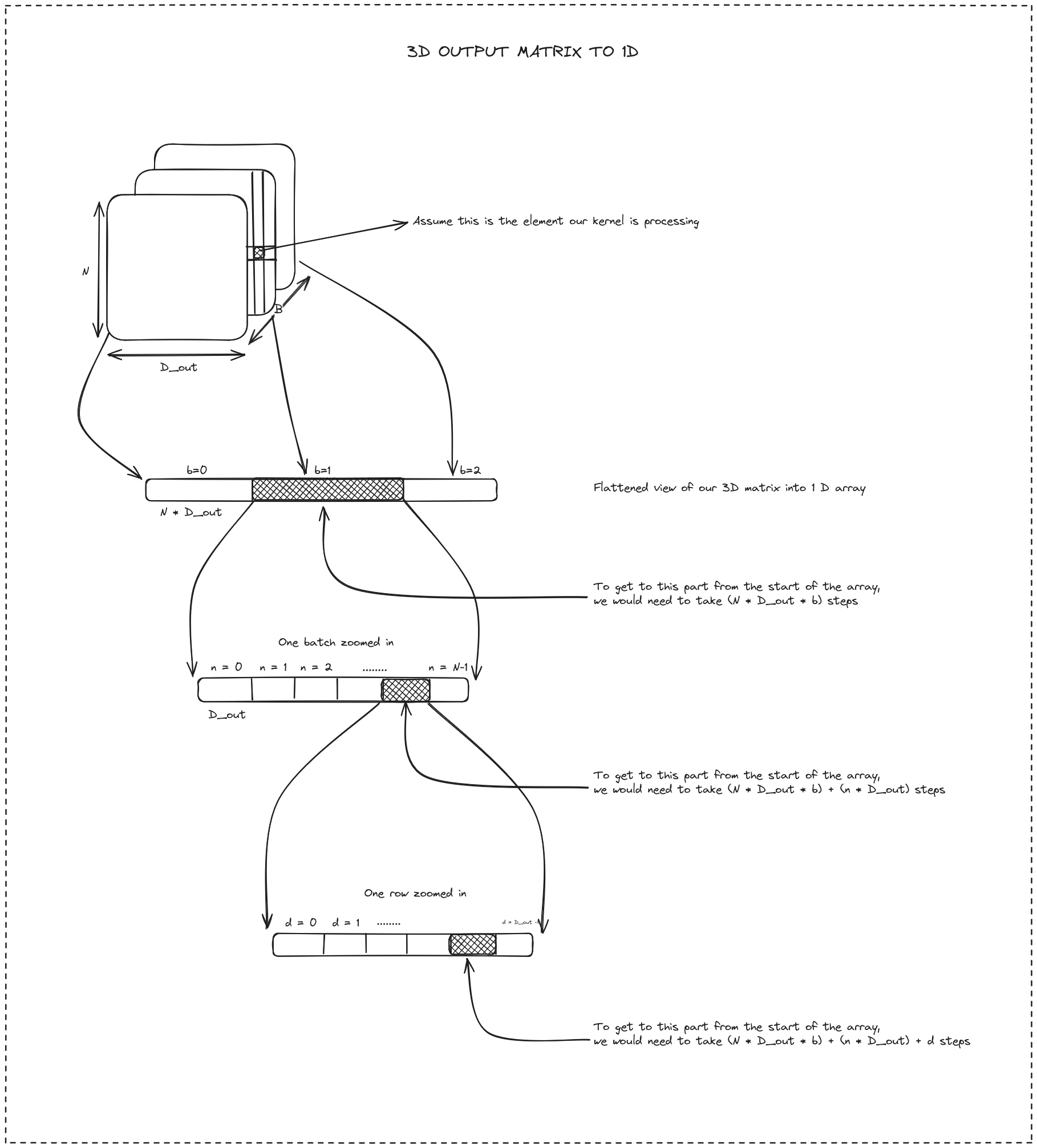
Figure 3: If the output data and threads have the exact length (which in this case is true), they can be mapped 1 to 1. B, N, D_out, are the batch size, number of rows, and number of columns in the output data respectively. b, n, d is i th batch, row, and column respectively.
After calculating these offsets, the corresponding row from X and the corresponding column from W are loaded followed by a single vector multiplication in a for loop. It is similar to out_offset calculation and should be easy to follow.
The complete code is present here. Running the code requires nvcc (the compiler for CUDA programs), an NVIDIA GPU to run the program, the CUDA drivers, and the CUDA toolkit installed.
A simple example in Triton
CUDA is amazing and allows a lot of optimizations. But it is quite verbose. Plus, it might not be comfortable for those coming from the machine learning or data science domain. Open AI released a package called Triton that provides a Python environment to write kernels and compile them for any GPU. Triton allows us to write very performant kernels in Python directly.
But instead of working with individual threads, Triton works with blocks. Instead of each kernel being assigned a thread, in Triton each kernel is assigned a block. Triton abstracts out the thread computation completely.
In the above example of matrix multiplication, instead of computing a single element of the output in the kernel, Triton can compute values for small “blocks” of the output matrix at once.
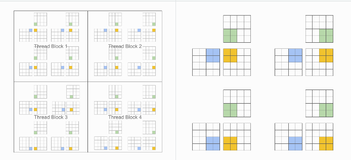
Figure 4: (Left) CUDA execution model vs (Right) Triton execution model Source: Triton documentation
Let’s reimplement the matrix multiplication example using Triton. The steps for Triton are very simple.
- Implement a “wrapper” function to call the kernel. Below, the Triton’s kernel is being called with
matmul_kernel. Define the grid and the block sizes similar to how it is done in CUDA. There are some assert statements to make sure that no errors are raised when input is passed to the kernel. Triton implicitly converts all torch tensors into a pointer. It just needs to be verified that all tensors passed to the kernel are already on the GPU (byx.to('cuda:0')).- Unlike CUDA however, the grid has 3 axes in this implementation. The first axis corresponds to the batch size, and in second axis corresponds to the number of times it will take
BLOCK_SIZE_ROWto cover all the rows (similarly forBLOCK_SIZE_COLfor the third axis). - During execution, this means, that for kernel will process -
BLOCK_SIZE_ROW x BLOCK_SIZE_COLsub-matrix in the input for every input in the batch.
- Unlike CUDA however, the grid has 3 axes in this implementation. The first axis corresponds to the batch size, and in second axis corresponds to the number of times it will take
def matmul(input: torch.Tensor, weight: torch.Tensor) -> torch.Tensor:
    """
    Implements matrix multiplication between two matrices. The input matrix is 3 dimension where
    first dimension is the batch size. The weight matrix will be multiplied with each of the batches
    of the input matrix.

    Args:
        input (torch.Tensor): Matrix with dimension (B x N x D_in)
        weight (torch.Tensor): Matrix with dimension (D_in x D_out)

    Returns:
        torch.Tensor: Ouptut matrix with dimension (B x N x D_out)
    """
    assert input.is_cuda, 'Inputs are not on GPU, ensure the input matrix is loaded on the GPU'
    assert weight.is_cuda, 'Weights are not on GPU, ensure the weight matrix is loaded on the GPU'
    assert input.shape[-1] == weight.shape[-2], 'Input and weight matrix are not compatible'

    B, N, D_in = input.shape
    _, D_out = weight.shape

    output = torch.empty((B, N, D_out), device=input.device, dtype=input.dtype)

    BLOCK_SIZE_ROW, BLOCK_SIZE_COL = 16, 16
    # Grid is aligned with the ouput matrix
    grid = lambda meta: (B, triton.cdiv(N, meta["BLOCK_SIZE_ROW"]), triton.cdiv(D_out, meta["BLOCK_SIZE_COL"]))

    matmul_kernel[grid](
        input_ptr=input,
        input_batch_stride=input.stride(0),
        input_row_stride=input.stride(1),
        input_col_stride=input.stride(2),
        weight_ptr=weight,
        weight_row_stride=weight.stride(0),
        weight_col_stride=weight.stride(1),
        output_ptr=output,
        output_batch_stride=output.stride(0),
        output_row_stride=output.stride(1),
        output_col_stride=output.stride(2),
        num_rows=N,
        num_input_cols=D_in,
        num_output_cols=D_out,
        BLOCK_SIZE_ROW=BLOCK_SIZE_ROW,
        BLOCK_SIZE_COL=BLOCK_SIZE_COL
    )

    return output
- That’s it. Tensor strides1 are used which is useful to figure out the step size needed between the next batch or row in the 1D flattened view of the 3D matrix. This will come in handy in the actual kernel. Once the kernel’s execution is complete, the output will be available in the tensor passed (
output).
The Triton kernel is decorated with a function @triton.jit for Triton to know that this is a function that will be executed on the GPU.
@triton.jit
def matmul_kernel(
    input_ptr,
    input_batch_stride,
    input_row_stride,
    input_col_stride,
    weight_ptr,
    weight_row_stride,
    weight_col_stride,
    output_ptr,
    output_batch_stride,
    output_row_stride,
    output_col_stride,
    num_rows,
    num_input_cols: tl.constexpr,
    num_output_cols,
    BLOCK_SIZE_ROW: tl.constexpr,
    BLOCK_SIZE_COL: tl.constexpr,
):
    # Getting block indexes in all 3 dimensions
    batch_idx = tl.program_id(0)
    row_idx = tl.program_id(1)
    col_idx = tl.program_id(2)

    # Offsets for input data
    input_batch_offset = batch_idx * input_batch_stride                                 # Offsets to reach to the correct batch. Similar to CUDA, but instead strides are being used here

    input_row_offset = row_idx*BLOCK_SIZE_ROW + tl.arange(0, BLOCK_SIZE_ROW)
    input_row_mask = input_row_offset[:, None] < num_rows
    input_row_offset = input_row_offset[:, None] * input_row_stride # Selecting relevant rows from input

    input_col_offset = tl.arange(0, num_input_cols)
    input_col_mask = input_col_offset[None, :] < num_input_cols
    input_col_offset = input_col_offset[None, :] * input_col_stride # Selecting all columns from input

    input_data_ptr = input_ptr + input_batch_offset + input_row_offset + input_col_offset
    input_data = tl.load(input_data_ptr, mask=(input_row_mask & input_col_mask)) # BLOCK_SIZE_ROW x D_in

    # Offsets for weight data
    weight_row_offset = tl.arange(0, num_input_cols)
    weight_row_mask = weight_row_offset[:, None] < num_input_cols
    weight_row_offset = weight_row_offset[:, None] * weight_row_stride # Selecing all rows from weight

    weight_col_offset = col_idx*BLOCK_SIZE_COL + tl.arange(0, BLOCK_SIZE_COL)
    weight_col_mask = weight_col_offset < num_output_cols
    weight_col_offset = weight_col_offset[None, :] * weight_col_stride # Selecting relevant columns from input

    weight_data_ptr = weight_ptr + weight_row_offset + weight_col_offset
    weight_data = tl.load(weight_data_ptr, mask=(weight_row_mask & weight_col_mask)) # D_in x BLOCK_SIZE_COL

    # Computation
    result = tl.dot(input_data, weight_data) # Matmul of a small block, BLOCK_SIZE_ROW x BLOCK_SIZE_COL

    # Offsets for output data
    output_batch_offset = batch_idx * output_batch_stride                               # Offsets to reach to the correct batch. Similar to CUDA, but instead strides are being used here

    output_row_offset = row_idx*BLOCK_SIZE_ROW + tl.arange(0, BLOCK_SIZE_ROW)
    output_row_mask = output_row_offset[:, None] < num_rows
    output_row_offset = output_row_offset[:, None] * output_row_stride

    output_col_offset = col_idx*BLOCK_SIZE_COL + tl.arange(0, BLOCK_SIZE_COL)
    output_col_mask = output_col_offset[None, :] < num_output_cols
    output_col_offset = output_col_offset[None, :] * output_col_stride

    output_data_ptr = output_ptr + output_batch_offset + output_row_offset + output_col_offset
    tl.store(output_data_ptr, result, mask=(output_row_mask & output_col_mask))
Similar to CUDA, calculate the current index of the block. But keep in mind, unlike CUDA where a single element of the output matrix is processed, here a single block (which is a 2D arrangement of a few elements) is processed. tl.program_id function helps in getting the index position in every axis.
batch_idxgets the output matrix in the batchrow_idxgets the block number along the rows. Remember, this is not equal to the row number as in CUDAcol_idxgets the block number along the columns. Remember, this is not equal to the column number as in CUDA
Once these 3 numbers are calculated, a 2D representation is created of the data that needs to be processed by each block. Let’s take some dummy numbers to understand how that is achieved. Assume that B = 1, N = 16, and D_out = 12. Block size in both column and row dimensions is 4 (i.e. BLOCK_SIZE_ROW and BLOCK_SIZE_COL is 4). So each block will be a 2D matrix of dimension (4 x 4).
Based on this
grid = lambda meta: (B, triton.cdiv(N, meta["BLOCK_SIZE_ROW"]), triton.cdiv(D_out, meta["BLOCK_SIZE_COL"]))
Based on the assumptions, the grid configuration is (1, 4, 3). A total of 12 blocks will be launched. Now, what would it take to load the block with rows 8 to 11 and columns 4 to 7? Based on simple arithmetic, it looks like (1, 2, 1)th block should be loaded where the first dimension corresponds to the batch dimension, the second dimension corresponds to the row dimension and the third dimension corresponds to the column dimension. This would correspond to
tl.program_id(axis=0) == 1
tl.program_id(axis=1) == 2
tl.program_id(axis=2) == 1
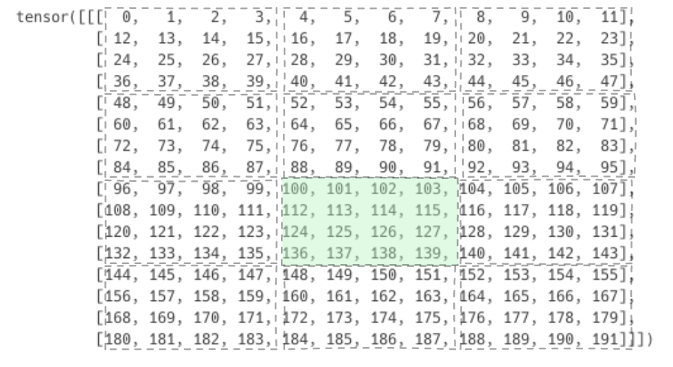
Figure 5: (1 x 16 x 12) matrix is divided into blocks of size (4 x 4). 1, 2, 1th block is highlighted. The value at every place is the index of that position in the 1D flattened array.
For this (1, 2, 1)th block, how to prepare the correct offsets? In the 1D representation of the matrix, the element numbers highlighted in green needs to be loaded.
# Offsets for output data
output_batch_offset = batch_idx * output_batch_stride

output_row_offset = row_idx*BLOCK_SIZE_ROW + tl.arange(0, BLOCK_SIZE_ROW)       # This arangement happens in 1D, tl.arange is like Python's arange
output_row_mask = output_row_offset[:, None] < num_rows                         # Think of masks as prevention against reading invalid data from memory
output_row_offset = output_row_offset[:, None] * output_row_stride              # This arangement converts a 1D vector to a 2D vector with (n, None) shape

output_col_offset = col_idx*BLOCK_SIZE_COL + tl.arange(0, BLOCK_SIZE_COL
output_col_mask = output_col_offset[None, :] < num_output_cols
output_col_offset = output_col_offset[None, :] * output_col_stride
Let’s decode what is happening here
output_row_offset = row_idx*BLOCK_SIZE_ROW + tl.arange(0, BLOCK_SIZE_ROW)
# row_idx = tl.program_id(1) = 2, BLOCK_SIZE_ROW = 4
# output_row_offset = 2*4 + (0, 1, 2, 3) = (8, 9, 10, 11)
If output_row_offset is added to the output_ptr directly the 8th, 9th, 10th, and 11th elements will be loaded from the 1D flattened array. But that is not desired. So how to get to the desired offsets:
output_row_offset = output_row_offset[:, None] * output_row_stride
# This multiplies each element by the output_row_stride which is equal to 12 (number of columns), the number of elements to skip in 1D array to reach the start of next row
# ouput_row_offset becomes (96, 108, 120, 132). It also gets transformed into a row vector
A similar transformation is done for the columns:
output_col_offset = col_idx*BLOCK_SIZE_COL + tl.arange(0, BLOCK_SIZE_COL)
# col_idx = tl.program_id = 1, BLOCK_SIZE_COL = 4
# output_col_offset = 1*4 + (0, 1, 2, 3) = (4, 5, 6, 7)
output_col_offset = output_col_offset[None, :] * output_col_stride
# This multiplies each element by the output_col_stride which is equal to 1, the number of elements to skip in 1D array to advance by one column.
# Since this is a row major ordering, columns are adjacent to each other.
# ouput_col_offset becomes (4, 5, 6, 7). It also gets transformed into a column vector
Finally,
output_data_ptr = output_ptr + output_batch_offset + output_row_offset + output_col_offset # Adds all the offsets to the pointer
First, add output_row_offset and output_col_offset. Since one of them is a row vector and the other is a column vector, on addition a 2D array is produced with all the desired indices of all the elements that need to be loaded. After that, add output_batch_offset to get to the correct matrix in the batch.
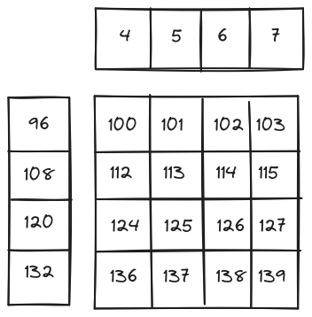
Figure 6: How 2D blocks are created from 2 1D offsets
This gives the appropriate offsets for the data this block is interested in computing. Similarly, the relevant data for the other two tensors can be computed. The core idea is understanding the block calculation and offset calculation. The rest of the code is more about syntax rather than any core logic.
The complete code is present here. Triton and PyTorch are needed to run this code.
How you can rewrite the complete architecture using optimized kernel
Congrats on making this far away. Now that you understand the basics of GPU hardware and its programming model, you can go ahead and implement any network from scratch, this time not relying on PyTroch for operations but writing your kernels in CUDA or Triton.
In case, you want to implement a transformer encoder network, you would need to implement all the basic layers and operations in Triton or CUDA.
- Matrix multiplication
- Layernorm
- Softmax
- Addition
- Concatenation
You can then wrap these kernels in the PyTorch module and load weights from HF to compare your implementation with other PyTorch/TF native implementations. If this sounds interesting, this is exactly what we did too. We implemented most of the operations used in Vision Transformer (ViT) including patching and addition operations in Triton and loaded weights from a checkpoint to run a forward pass. You can look at the code at ViT.triton and maybe implement your favorite model too using custom kernels!
Citations
For attribution, please cite this as
@article{romit2024gpus2,
  title   = {GPUs Part 2},
  author  = {Jain, Romit},
  journal = {cmeraki.github.io},
  year    = {2024},
  month   = {May},
  url     = {https://cmeraki.github.io/gpu-part2.html}
}